
Differential expression analysis
Differential expression analysis allows you to determine which genes are expressed at different levels between experimental groups. Differentially expressed genes can then be used in pathway analysis to offer insight into the biological processes affected by the condition of interest.
Using Trailmaker, you can find the differential expressed genes between two groups of cells, where each group must have at least 3 cells. Differential expression can be calculated using the differential expression tab on the right side in the ‘Genes’ block.
Differential expression results in Trailmaker are computed on log-normalized expression values.
Reported log fold changes (logFC) reflect differences in log-normalized counts between the groups being compared, rather than raw transcript counts.
You can compare cell sets within a sample/group, which allows you to find marker genes that distinguish clusters from one another.
Alternatively, you can compare a selected cell set between samples/groups to find genes that are differentially expressed between two experimental groups.
Compare cell sets within a sample/group
The differential expression calculation to compare cell sets within a sample or group uses the presto implementation of the Wilcoxon rank sum test and auROC analysis. For more information see the presto vignette.
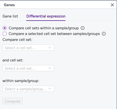
To perform this analysis, choose a cell set you want to compare in the first drop-down menu. Choose another cell set, the option ‘Rest of Louvain clusters’ or ‘All other cells’ in the second drop-down menu. [Note that in the case of Louvain clusters, ‘Rest of Louvain clusters’ and ‘All other cells’ is the same because all cells are assigned to a Louvain cluster; whereas for Custom cell sets, these two options will be different if not all cells in the dataset are assigned to a Custom cell set.] Lastly, select the sample/group within which you want to compare cell sets or choose the option ‘All’. Then click compute.
You will be presented with the differential expression (DE) results table: a list of genes in descending order of log fold change (logFC). The table returns the following results:
- LogFC: The fold change is the ratio of the expression of a gene between the two groups being compared. They are then log-transformed in base2. Genes with a positive logFC that appear at the top of the list are expressed at higher levels in the comparison group A compared to group B. Given that logFC = log2(A) - log2(B), if log2(A) is negative and log2(B) is positive, then the logFC will be positive.
- Adj p-value: The probability of observing the difference in expression for a given gene under the assumption that said gene is not differentially expressed. In addition, the value is adjusted using the Benjamini–Hochberg correction for multiple hypothesis testing, to account for the fact that when testing thousands of genes, some might have a small p-value due to random chance. The smaller it is, the higher the chance the gene is actually differentially expressed.
- Pct1: The percentage of cells where the gene is expressed in the first group (A).
- Pct2: The percentage of cells where the gene is expressed in the second group (B).
- AUC: Area under the receiver operating characteristic (ROC) curve. It is proportional to the Wilcoxon U statistic calculated by the rank-sum test. The larger it is, the more likely it is that the corresponding gene is differentially expressed.
- Note that average expression is not output from the Presto vignette.
- Note that in Scanpy projects the Wilcoxon rank sum test (used for "within" sample/group comparisons) is run on the top 5,000 highly variable genes. Genes outside this set are not tested and will not appear in the results.
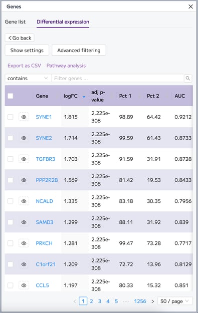
The DE gene list can be reordered in the table by other calculated parameters - adjusted p-value, PCT 1 (the percentage of cells where the feature is detected in the first group), PCT 2 (the percentage of cells where the feature is detected in the second group), and AUC (area under the receiver operating characteristic curve). Both ascending and descending options are available to view.
Clicking on ‘Show settings’ will show your chosen cell sets and samples/groups that have been compared in this DE calculation.
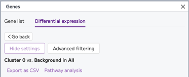
Note that to download the DE results, you must visit the Volcano plot in the Plots and Tables module. Unfortunately, the DE results table cannot be downloaded from the Data Exploration module.
Compare a selected cell set between samples/groups
The differential expression comparison of a selected cell set between samples or groups uses a pseudobulk limma-voom workflow. This is considered best practice for between sample comparisons. Pseudo-bulk differential expression sums the counts for all cells within a cluster for each sample and then uses standard differential expression methods designed for bulk RNA-seq. One major benefit to doing this is that it treats the sample as the level of replication, instead of falsely assuming that each cell is independent.
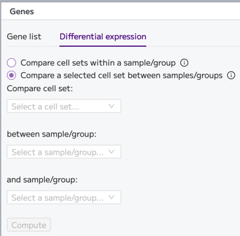
To perform this DE analysis, choose a cell set you want to compare in the first drop-down menu. Choose the first sample/group to compare in the second drop-down menu. Lastly, select the second sample/group you want to compare with the first sample/group or choose the option ‘Rest of Samples’ or ‘All other cells’. When you have made your selections for the DE calculation parameters, click ‘Compute’.
Note that in some comparison selections, this warning message will appear:
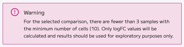
The message explains that in your selected comparison, there are fewer than 3 samples with the minimum number of cells that’s required to perform the DE calculation. The most likely explanation is that you are comparing 1 sample to 1 other sample. An alternative explanation is that you are comparing 3 or more samples, but that there are too few cells (<10) in one or more of the comparison groups, which is resulting in only 2 ‘valid’ comparison groups that contain enough cells to perform the DE calculation.
In this case, you can still go ahead and perform the DE calculation, but the DE results table will only display the list of DE genes and logFC value. No adjusted p-value will be calculated as it is not considered statistically sound to calculate such a p-value on a 1 versus 1 comparison.
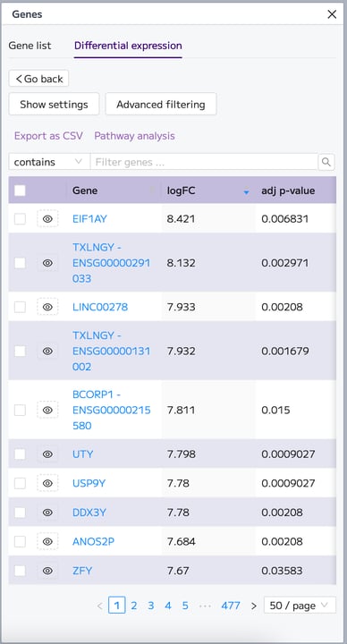
You will be presented with the differential expression (DE) results table: a list of genes in descending order of log foldfull change (logFC).
The table returns the following results:
- If the comparison contains 3 or more samples (e.g. 2 control vs 1 treated) then the DE results table presents both the logFC and the adj p-value. In this case, the p-values generated from pseudo-bulk comparisons are statistically accurate and can be used to determine biological significance. The p-value is adjusted using the Benjamini–Hochberg correction for multiple hypothesis testing, to account for the fact that when testing thousands of genes, some might have a small p-value due to random chance. The smaller it is, the higher the chance the gene is actually differentially expressed.
- For 1 vs 1 comparisons (e.g. 1 control vs 1 treated), only the logFC is returned in the results table, because p-values are not appropriate with this small N. LogFC estimates can be used to ascertain the magnitude of the difference between the two samples but not to draw any statistical inferences.
For further guidance, see Performing differential expression between samples or groups in Trailmaker.
The gene list can be reordered in the table by other calculated parameters by clicking on the column titles.
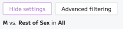
Clicking on ‘Show settings’ will show your chosen cell sets and samples/groups that have been compared.
Advanced filtering
To filter the DE gene list, click ‘Advanced filtering’.
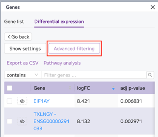
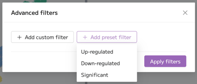
In the popup menu, you can select advanced filtering options. There are three pre-set filtering options which allow you to quickly filter for only the up-regulated genes (with a positive logFC), only the down-regulated genes (with a negative logFC) or only the significant genes (with an adjusted p-value of <0.05):
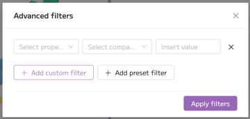
Alternatively, you can add your own custom filter using the ‘Add custom filter’ option. Here, you can select to filter by any of the DE results parameters and set a filtering threshold of your choice.
Pathway enrichment analysis
Pathway analysis identifies biological pathways that are enriched in the differentially expressed gene list more than would be expected by chance. The goal is to give the list of genes across different phenotypes a biological context by condensing down a potentially long list of genes into a few select biological pathways.
Click ‘Pathway analysis’ after performing differential expression, to start your pathway analysis. We strongly recommend using Advanced filtering to filter your list of DE genes before performing pathway analysis. This is because the list of differentially expressed genes is very long and contains both up- and down-regulated genes with varying levels of significance. So, further filtering will lead to more consistent and clear pathway analysis results.
Once your list of DE genes has been filtered using the ‘Advanced filtering’ tool, select ‘Pathway analysis’ to begin:
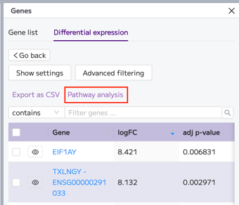
Note that if you have not already filtered your gene list, you will be prompted to do so.

Pathway analysis can be performed on a list of differentially expressed genes using the external service providers PantherDB or Enrichr. The list of genes and species will be submitted to the external service, and no other information will be sent.
We recommend running your pathway analysis using both PantherDB and Enricher and then comparing the results. Your final choice for the pathway analysis service might depend on the databases in the platforms, user interface, and, ultimately, on your personal preference.
For help using these external pathway analysis services, we recommend visiting the Help pages for PantherDB and Enrichr.
PantherDB
Select the ‘pantherdb’ toggle at the top of the pathway analysis modal:
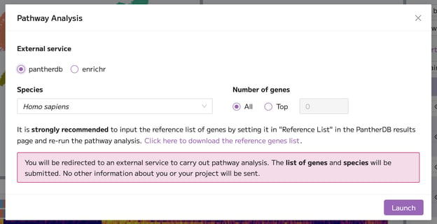
In the pathway analysis modal, you can confirm the species of your dataset. You can also select the number of differentially expressed genes that will be included in the pathway analysis by clicking ‘Top’ and inputting the desired number. To send all the genes in your filtered list, select ‘All’.
Then, initiate your pathway analysis by clicking ‘Launch’.
PantherDB is hosted on an unsecured server (HTTP), so you will see a warning upon launch. Click “Send anyway” to continue. The list of genes and species will be submitted to the external service, and no other information will be sent. See the example below.

You will be redirected to the PantherDB website in a new tab.
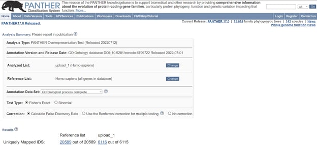
We recommend inputting the reference list of genes by setting it in "Reference List" on the PantherDB results page and re-run the pathway analysis. If gene names in Trailmaker are different than in the reference list of genes on PantherDB (for instance, lowercase vs. uppercase gene names), the results of pathway analysis will be incorrect.
For further help using PantherDB, please visit the relevant help pages on the PantherDB website: http://pantherdb.org/help/PANTHERhelp.jsp.
Enrichr
Enrichr is available for both Seurat and Scanpy projects. Within the Pathway Analysis modal, select ‘enrichr’.
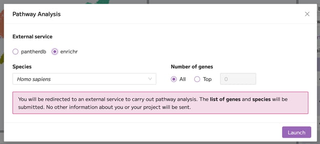
In the pathway analysis modal, you can confirm the species of your dataset. You can also select the number of differentially expressed genes that will be included in the pathway analysis by clicking ‘Top’ and inputting the desired number. To send all the genes in your filtered list, select ‘All’.
Then, initiate your pathway analysis by clicking ‘Launch’.
You will be redirected to the maayanlab.cloud Enrichr page in a new tab.
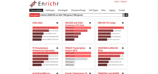
For further help using the Enrichr pathway analysis tool, please visit the relevant help pages on the Enrichr website: https://maayanlab.cloud/Enrichr/help.
Data Exploration for immune repertoire analysis
Paired WT+immune projects
The Data Exploration page is enabled for paired WT and immune (WT+TCR or WT+BCR) projects.
For immune projects in Trailmaker, a Clonotype List is displayed as a separate tab next to the Gene List on the right side of the Data Exploration view.
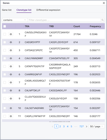
The clonotype list displays all identified clonotypes in the dataset, in descending order of frequency across all samples. The clonotype list includes the following columns:
- Clonotype ID (column 1) is assigned to clonotypes according to frequency across the whole dataset. The most abundant clonotype is assigned to clonotype ID 1.
- The clonotype’s primary chain sequences are available in columns 2 and 3. For TCR data, the chains are TRA and TRB, while for BCR data the chains are IGK/L and IGH.
- Count indicates the number of cells identified with each clonotype across all samples in the dataset.
- Frequency illustrates the abundance of each clonotype across all samples in the dataset. The clonotype list is ordered in descending order of frequency.
From the clonotype list, individual clonotypes can be overlaid on the UMAP using the eye icon.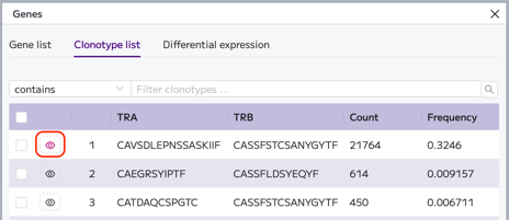
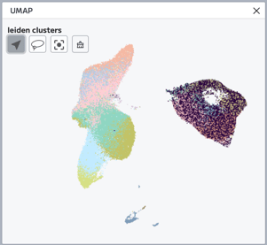
The selected clonotype will be shown in the UMAP in navy. The non-focus cells will remain colored by Leiden clusters (if selected) or will appear in grey. Other cell set coloring of the UMAP, such as Leiden clusters, can be cleared from the UMAP by clicking the eye icon next to the relevant cell set family in the Cell sets and Metadata tile.
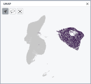
To overlay multiple clonotypes on the UMAP, select the relevant clonotypes of interest using the check boxes and click ‘Color UMAP’.
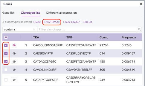
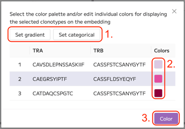
In the modal that appears, the default color settings can be set as a gradient or categorical (1.) and the colors of individual clonotypes can be customized (2.). Click ‘Color’ to color the UMAP (3.).
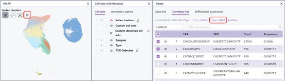
To clear multiple clonotype colors from the UMAP, select ‘Clear UMAP’ or use the paintbrush in the UMAP tile.
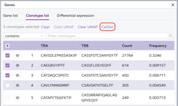
To create a custom clonotype cell set, select the relevant clonotypes of interest from the clonotypes list, then click ‘CellSet’. The new cell set will appear in the ‘Custom clonotype cell set’ family in the Cell sets and Metadata tile. The Custom clonotype cell set can be renamed, recolored or deleted as per the behaviour of the Custom cell sets.
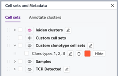
With Custom clonotype cell sets, it’s then possible to utilize the other functionality within the Cell sets and Metadata tile, including hide, combine/intersect/complement, and subset to a new analysis. See this section of the user guide for more details. Note that the clonotype IDs will be regenerated during subsetting of immune projects, which will potentially result in different clonotype IDs for a given clonotype with specific chains of interest.
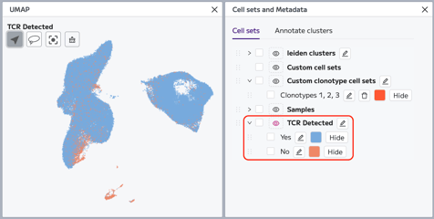
In the Cell sets and Metadata tile the ‘TCR Detected’ (for TCR datasets) or ‘BCR Detected (for BCR datasets) is included automatically in all paired WT+immune projects. All cells in the dataset are included in this cell set family, grouped as Yes or No. Cells in the ‘Yes’ group have an identified paired TCR or BCR clonotype.
Immune only projects
The Data Exploration page is disabled for Immune only (TCR or BCR data without a WT parent) projects.