Data Exploration

Overview

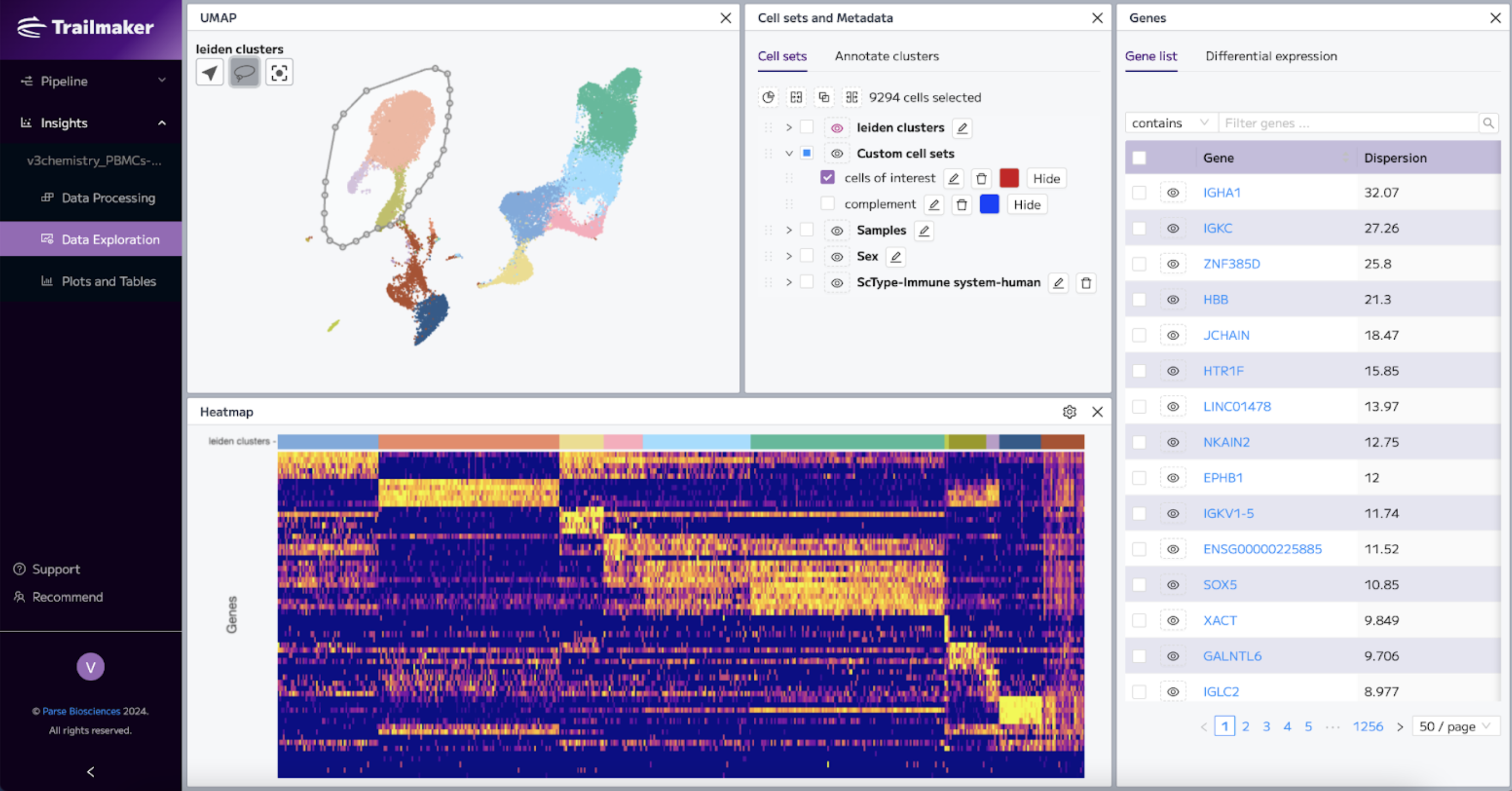
The Data Exploration tab within the Insights module of Trailmaker has a wide variety of features for in-depth exploration of your data. Using this module, users can identify which cell types are represented by their cell sets, fully customize cell set selection, and generate insight into the dataset using gene expression visualization and differential expression.

Custom cell sets can be created using selection tools, based on the expression of one or more genes, or by manipulating the default Leiden or Louvain clusters. It's easy to rename clusters or recolor by sample, metadata, or gene. Standard analysis actions such as marker heatmap and UMAP are pre-loaded. Cell set annotation can be done automatically, or manually using the marker heatmap and differential expression features.

Users can calculate differential expression between cell sets within a sample/group or compare a cell set between samples and groups. Differential expression results can be filtered further, for example, by selecting only upregulated genes. Users can perform pathway analysis on the list of differentially expressed genes using external services - Pantherdb or Enrichr.

Navigation

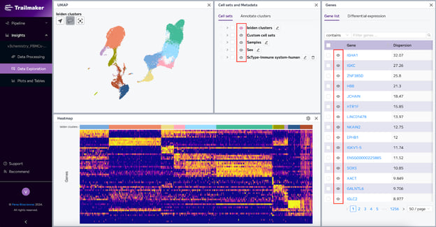
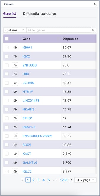
The Data Exploration tab consists of several tiles. On the top left, we have the UMAP embedding that was created and customized in step 7 of the Data Processing (1). In the middle, we have the list of default clusters (Leiden or Louvain), any custom cell sets that have been created, as well as the list of samples and metadata (2). On the right, the gene list shows the full list of genes present in the dataset ordered by dispersion (3). Dispersion is a measure of variability, so some of the most variable genes in the dataset are listed at the top of the gene list. At the bottom, the heatmap shows marker genes for your selected clustering method (Leiden or Louvain) (4).

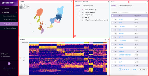
The width and height of different tiles can be changed to suit your preference. The tiles can also be moved around using the moving arrows , and closed using the X button on the top right corner of each tile. To get to the default layout of the Data Exploration module back again, refresh the page or click on another module and then back to the Data Exploration.

Note that plot download is not available in the Data Exploration module. All plots, including the UMAP or t-SNE embedding and the heatmap, can be fully customized and exported in various formats from the Plots and Tables module.

Cell sets and Metadata tile

In the Cell sets and Metadata tile, there are two tabs: 'Cell sets' where you find the lists of all cluster families, samples and metadata groups; and the 'Annotate clusters' tab where you can perform automatic annotation.

Cell counts

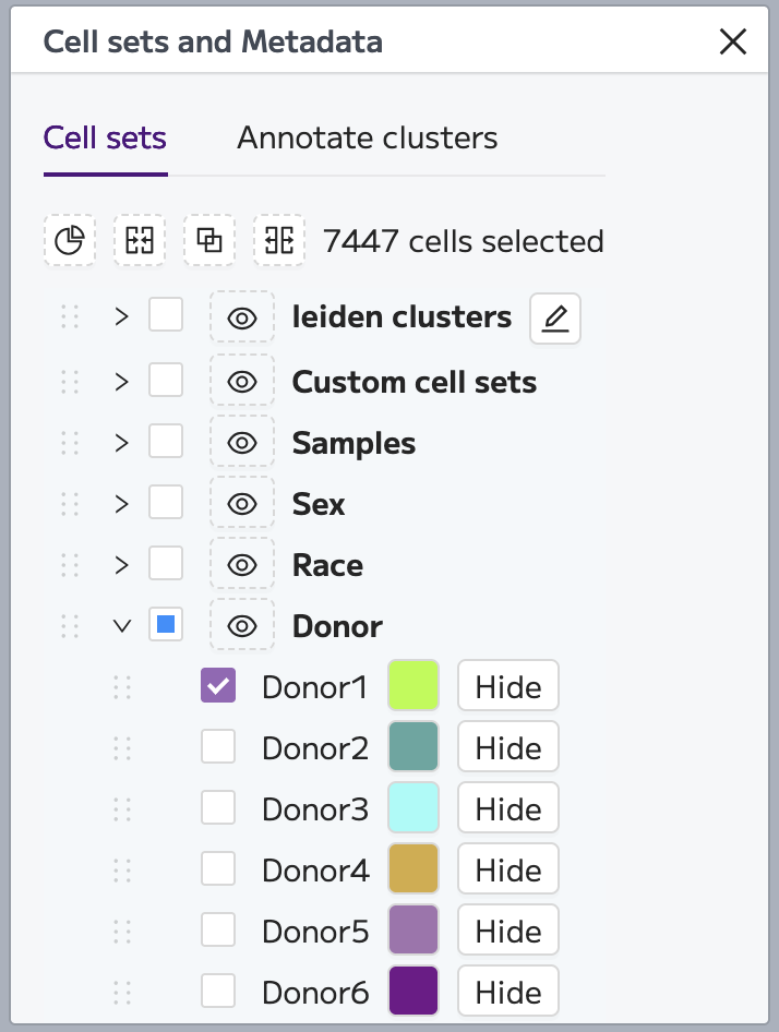
To find the post-filtering cell counts for individual cell sets, samples or metadata groups, use the check boxes in the Cell sets and Metadata tile. By selecting one checkbox, the cell count for the selected cell set, sample or metadata group is shown at the top of the box. In this example, "7447 cells are selected". When multiple boxes are checked, the sum cell count is shown.

Viewing cell sets

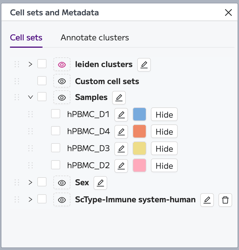
The ‘Cell sets’ tab shows the list of the default clusters (Leiden or Louvain) and any custom cell sets that have been created, as well as the list of samples and metadata. To expand any of the lists, click on the arrow on the left of the list name.

Changing names and colors of cell sets

In Leiden/Louvain clusters, Custom cell sets lists, ScType annotated cell sets, samples and metadata in the Cell sets and Metadata tile, you can change the names and colors of cell sets.

To change the name click the edit button next to the cell set name. After inputting the new name, click the checkmark to save the name or the cross to cancel. Any changes to cell set names made in this tile propagate all other modules of the platform.

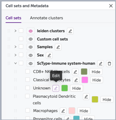
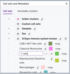
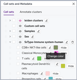
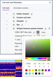
To change the color of a cluster, click on the colored circle next to the cell set. In the popup, choose the new color and it will be applied automatically. Any changes to cell set colors made in this tile propagate all other modules of the platform.

Reordering cell sets

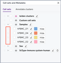
It’s possible to rearrange the order of cell set and group lists. To reorder a cell set or group list, drag an item to the desired position using the button (3 lines) on the left of the item name. The new order of cell sets or groups in the Cell sets and Metadata block will be then represented in the heatmap in the Data Exploration module, as well as all plots in the Plots and Tables module. This is a useful feature for ensuring that your samples, metadata groups and annotated cell sets are plotted in order that you want them to be.

Performing automatic annotation

The ‘Annotate clusters’ tab within the Cell sets and Metadata tile is where you can perform automatic cluster annotation. For Seurat projects the automatic annotation option is ScType, while for Scanpy projects the two automatic annotation options are Decoupler and CellTypist.

The ScType method (Seurat) of automatic annotation uses a marker genes database which was built using CellMarker, PanglaoDB, and 15 novel cell types with corresponding marker genes added by manual curation of more than 10 papers. The current version of the ScType database contains a total of 3,980 cell markers for 194 cell types in 17 human tissues and 4,212 cell markers for 194 cell types in 17 mouse tissues. More details can be found in the original paper and in the ScType github repository.
The Decoupler method (Scanpy) of automatic annotation uses the Overrepresentation Analysis (ORA) method implemented in decoupler-py. ORA measures the overlap between a target feature set (the marker genes in the PanglaoDB database) and the marker genes of a given experiment. With these, a contingency table is built and a one-tailed Fisher's exact test is computed to determine if a cell type's set of features are over-represented in the selected features from the data. More details can be found in the decoupler documentation, and in the original paper.
The CellTypist method (Scanpy) of automatic annotation uses an automated scRNA-seq annotation tool based on regularised logistic regression classifiers. More details can be found in the CellTypist website or in the original paper.

To perform automatic annotation, select the method (if relevant) and input the species and tissue tissue type using the dropdown menus. Then click ‘Compute’.

Note that the method selection options are enabled/disabled based on whether the project uses Seurat or Scanpy (see Step 6: Data integration), and the ‘Compute’ button is disabled until the dropdown menu selections are complete.

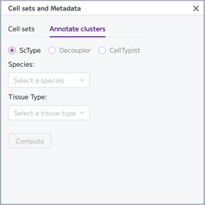
The annotated clusters appear in a new cell set within the Cell sets tab, labelled according to the annotation method used.

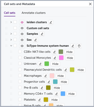
For further guidance on cell type annotation, see: How to annotate cell types in Trailmaker.

Creating custom cell sets

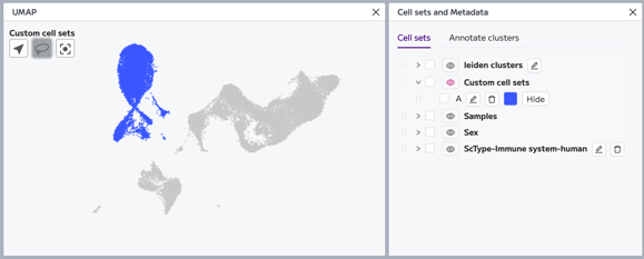
Creating custom cell sets using the lasso tool in the UMAP

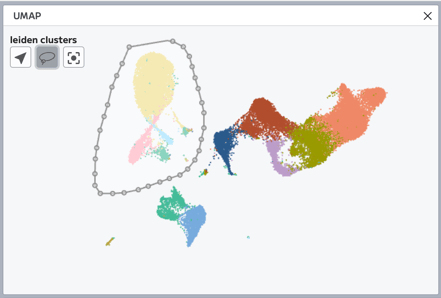
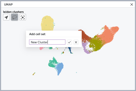
New cell sets can be created using the lasso selection tool in the UMAP (or t-SNE) embedding plot. The lasso tool allows for a precise selection of an area of cells in your UMAP embedding plot. You can name the new cell set. The new cell set will appear in the ‘Custom cell sets’ list in the Cell sets and Metadata tile. To see the new cell set colored in UMAP, click on the eye icon next to ‘Custom cell sets’.

Custom cell sets based on gene expression

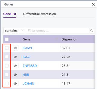
You may want to create a new custom cell set based on the expression (or lack of expression) of one or more genes. In the gene list on the right-hand side of the Data Exploration tab, you can select one or more genes of interest using the checkboxes next to the genes.

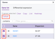
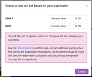
By selecting genes and clicking the 'Cellset' button, you can generate a new cell set based on the raw expression of the selected genes. In the Cellset modal, set the thresholds of expression for each selected gene. For example, you can select only the cells that express a particular gene at very high levels; or you can select only the cells that lack expression of selected genes.

Given that raw gene expression values can vary a lot depending on the gene, the thresholds for creating cell sets based on gene expression should be selected carefully for each gene based on viewing the raw expression for each individual gene in the Violin plot.

Then click ‘Create’. Your new cell set will appear in the Custom cell sets list in the Cell sets and Metadata tile. To see the new cell set colored in UMAP, click on the eye icon next to ‘Custom cell sets’.

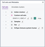
Custom cell sets of combined Leiden or Louvain clusters

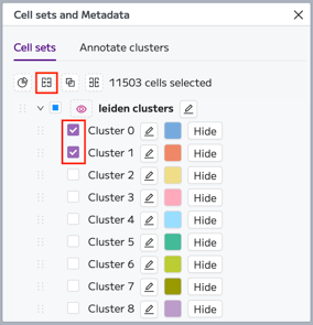
Locate the list of Leiden or Louvain clusters in the Cell sets and Metadata tile. Select two or more clusters that you would like to combine using the checkboxes next to cluster names. Then click the ‘Combine’ button. In the popup, name the new cluster and click on the tick button to save.

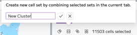
The new cluster will appear in the ‘Custom cell sets’ list.

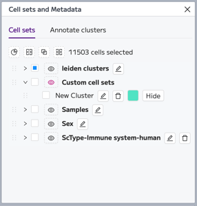
Note that if you want to copy over all your other Leiden or Louvain clusters to the Custom cell sets list, you can do so using the 'Combine' button with only one cluster selected at a time. This essentially copies the selected Leiden or Louvain cluster to the Custom cell sets list.

Intersect selected cell sets

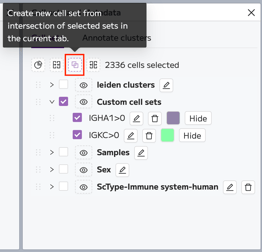
Intersecting selected cell sets can be very useful when working with non-mutually exclusive cell sets. For example, you’ve created two new cell sets based on gene expression. Cell set 1 contains cells with gene expression of Gene 1 greater than 0.10, and cell set 2 contains cells with gene expression of Gene 2 less than 1. Now, there might be some cells in both of these new cell sets that are the same - with gene expression of Gene 1 greater than 0.1 and Gene 2 less than 1. Intersecting cell set 1 and cell set 2 will highlight cells present in both cell sets and combine them in a new cluster.

To use this function, locate the list of clusters in the Cell sets and Metadata tile. To create an intersection of cells, select clusters using the checkboxes next to cluster names. Then click the ‘Intersection’ button. In the popup, name the new cluster and click on the save button. The new cluster will appear in the ‘Custom cell sets’ list.

Create a new custom cell set from the complement of selected cell sets

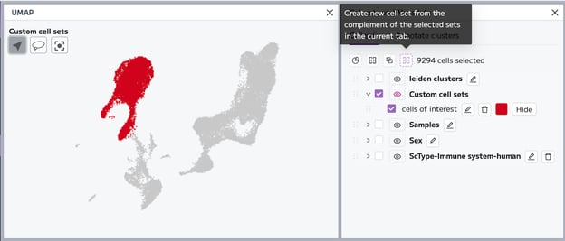
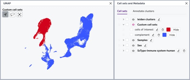
Using this function, you can create a new custom cell set that contains all cells that are not in the selected cluster(s). This can be useful and time-saving when you have many clusters and want to create a cell set with all cells outside of these clusters.

Select the cell set(s) that you want to create a complement of, and click the “Complement” button. In the popup, name the new cluster and click on the save button. The new cluster will appear in the ‘Custom cell sets’ list. To see the new cell set colored in the UMAP, click on the eye icon next to ‘Custom cell sets’.

Subset selected cell sets to a new project

You can create a new project by subsetting (also known as sub-clustering or reclustering) a cell selection from your project. This allows for a further deep dive into part of your data and the removal of unwanted clusters (such as unknown cells or contamination) from your project.

When you have made a selection of a group of cells, a subset button appears in the Cell sets and Metadata tile.

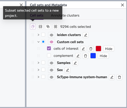
When you click on the subset button, a pop-up appears to start a new project from your current cell selection. You can change the name of the new project, if you wish. Then click ‘Create’, to make a new project containing your selection.

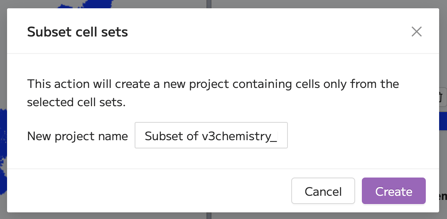
Data Processing is run for this subset project, after which you can start your deep dive in the Data Exploration module for the subset of cells.

UMAP or t-SNE embedding tile

The tile on the top left of the Data Exploration module shows the embedding - UMAP or t-SNE - that was customized in step 7 of Data Processing. UMAP is shown by default. To change between UMAP and t-SNE, go back to step 7 of Data Processing to change your selection. The embedding plot in the Data Exploration module is interactive, allowing you to zoom in and out to focus on a particular area of interest, move, and hover over single cells.

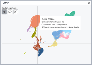
Hovering over a single cell gives you information about the cell ID and the cluster the cell belongs to, with the selected cell simultaneously highlighted in the marker heatmap.

Viewing genes on the UMAP or t-SNE embedding

The embedding is colored by Leiden or Louvain clusters by default. The coloring of the embedding can be changed using the ‘eye’ icons throughout the Data Exploration tab, for example to visualize samples or metadata, or the expression of a single gene from the gene list. Note that when cell sets are viewed on the embedding, cells that are not assigned to a cell set appear in gray.

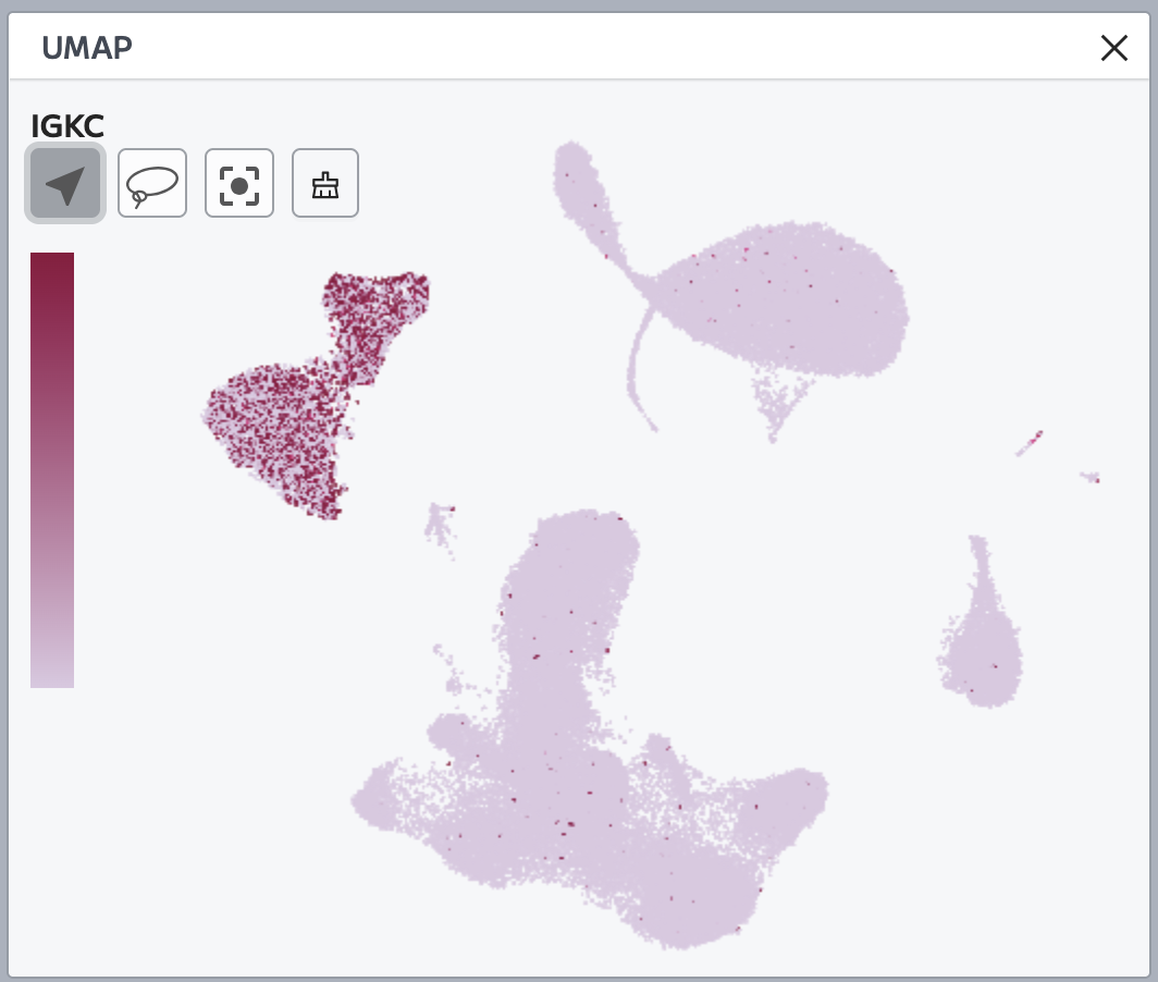
Below is an example of the UMAP colored by a selected gene using the 'eye' icon from the Gene list. This plot is often referred to as a feature plot:

The UMAP plot also allows the creation of new custom cell sets by using the lasso tool.

Heatmap

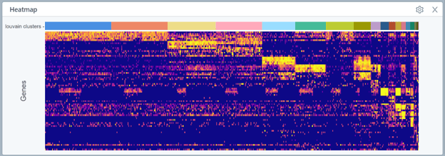
The heatmap shows marker genes for the Leiden or Louvain clusters by default. Marker genes have been calculated using a Wilcoxon rank-sum test (wilcoxauc from the presto package in Seurat or sc.tl.rank_genes_groups in Scanpy). The heatmap displays log-normalized expression values.

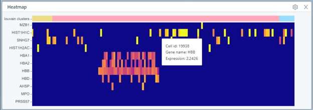
The number of genes shown per cluster varies depending on how many clusters you have in your dataset. You can zoom in on a specific cell set of interest in the heatmap, and hover over marker genes to identify the gene name which will help to identify the represented cell type.

The heatmap settings menu is accessed by clicking on the gear/cog icon. In this menu, you can add sample/metadata tracks to the heatmap view or reorder the heatmap, as explained below.

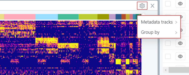
Adding sample/metadata track to the heatmap view

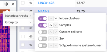
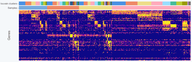
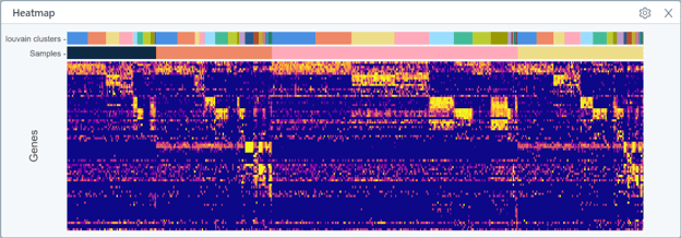
To add sample or metadata tracks to the heatmap view, hover over Metadata tracks in the heatmap settings menu. In the sub-menu, toggle the eye icon to add a metadata track. The toggled selections appear as colored tracks above the heatmap view. The order of the metadata tracks can be changed by clicking on the up and down arrows. The item on top of the list is also going to be shown at the top of the heatmap tile. Note that this doesn’t reorder the cells within the heatmap itself - this is done using the ‘Group by’ function (see the next section).

Reordering the cells on the heatmap using ‘Group by’ parameter

To reorder the cells viewed in the heatmap, hover over ‘Group by’ in the settings menu. In the sub-menu, hover over ‘Select the parameters to group by’ dropdown menu. Click + to add a parameter you want to order cells by. To exclude a parameter, click - on the left of the parameter.

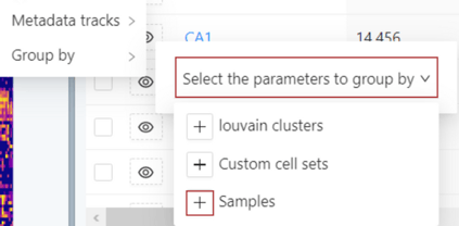
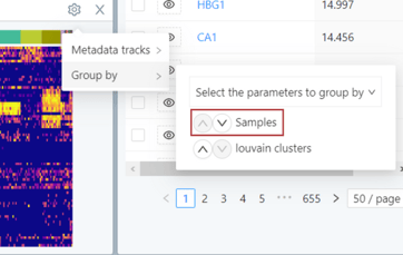
Then, in the ‘Group by’ sub-menu, arrange the parameters in descending order by which you would like to group them by.

In the example below, the heatmap is ordered first by sample and then by Louvain clusters:

Viewing genes in the heatmap

You can search for specific genes of interest in the gene list. If you want to look at these genes in the heatmap, you can select them using the checkbox and click ‘Heatmap’.

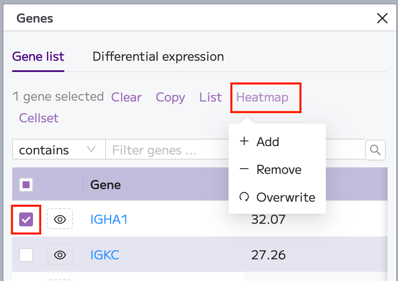
This gives you an option to add or remove the selected genes from the heatmap or overwrite the heatmap with the selected genes(s).

Clicking remove will remove the selected gene(s) from the heatmap. Clicking add will add the selected gene(s) to the heatmap.

Using overwrite, the heatmap only shows the expression of the selected gene(s). If at any point you want to reload the default heatmap view showing marker genes, simply reload the page.

Hiding Cell Sets

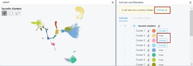
You can hide one or more clusters, samples, or metadata groups from the embedding plot and heatmap.

To hide a particular cluster from the embedding plot and heatmap, click the Hide button on the right side of the cluster name in the Cell sets and Metadata tile. To unhide a cluster or clusters, click the ‘Unhide’ button or use ‘Unhide all’ to unhide all hidden clusters. Metadata groups and Samples can also be hidden/unhidden in this way.

Gene list

You can find the full Gene list for your dataset in the ‘Genes’ tile on the right-hand side of the Data Exploration module. By default, genes are presented in descending order by dispersion. Dispersion describes how much the variance deviates from the mean. Genes with high dispersion have a high level of variation between cells in the dataset. You can rearrange the gene list based on the gene name or dispersion by clicking on the column names (Gene and Dispersion).

Note that if you use SCTransform, the number of genes displayed in the Gene List may be lower than the total number of genes originally detected in your dataset. Further information on gene filtering when using SCTransform is provided in Step 6: Data Integration.

Search for genes in the gene list

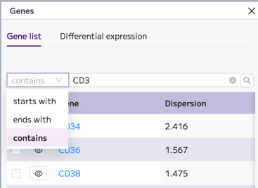
You can search for genes that contain, start with or end with certain letter/s or possible subunits. Your search is applied automatically to the gene list as you type.

To clear a gene search, delete your input in the search box or click the cross button (✖) on the left of the search box.

Viewing gene information

If you want to view information on a particular gene in the Gene List, click on the gene name. This action opens a new window showing the selected gene in GeneCards.

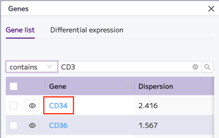
Note that the GeneCards database is used primarily for human genes and may not provide useful information if your dataset is from a species other than human.

Trailmaker User Guide: Data Exploration (part 1)